Welcome

How to Cite This Book

If you use this book in your work, please cite it as:

APA: Chaudhri, A. (2026). Real-Time Supply Chain Routing with Neo4j, Snowflake Postgres and Confluent Kafka. Self-published. https://realtime-supply-chain.github.io/

BibTeX:

@online{chaudhri2026supplychain,
  author  = {Chaudhri, Akmal},
  title   = {Real-Time Supply Chain Routing with Neo4j, Snowflake Postgres and Confluent Kafka},
  year    = {2026},
  url     = {https://realtime-supply-chain.github.io/},
  urldate = {2026-09-13}
}

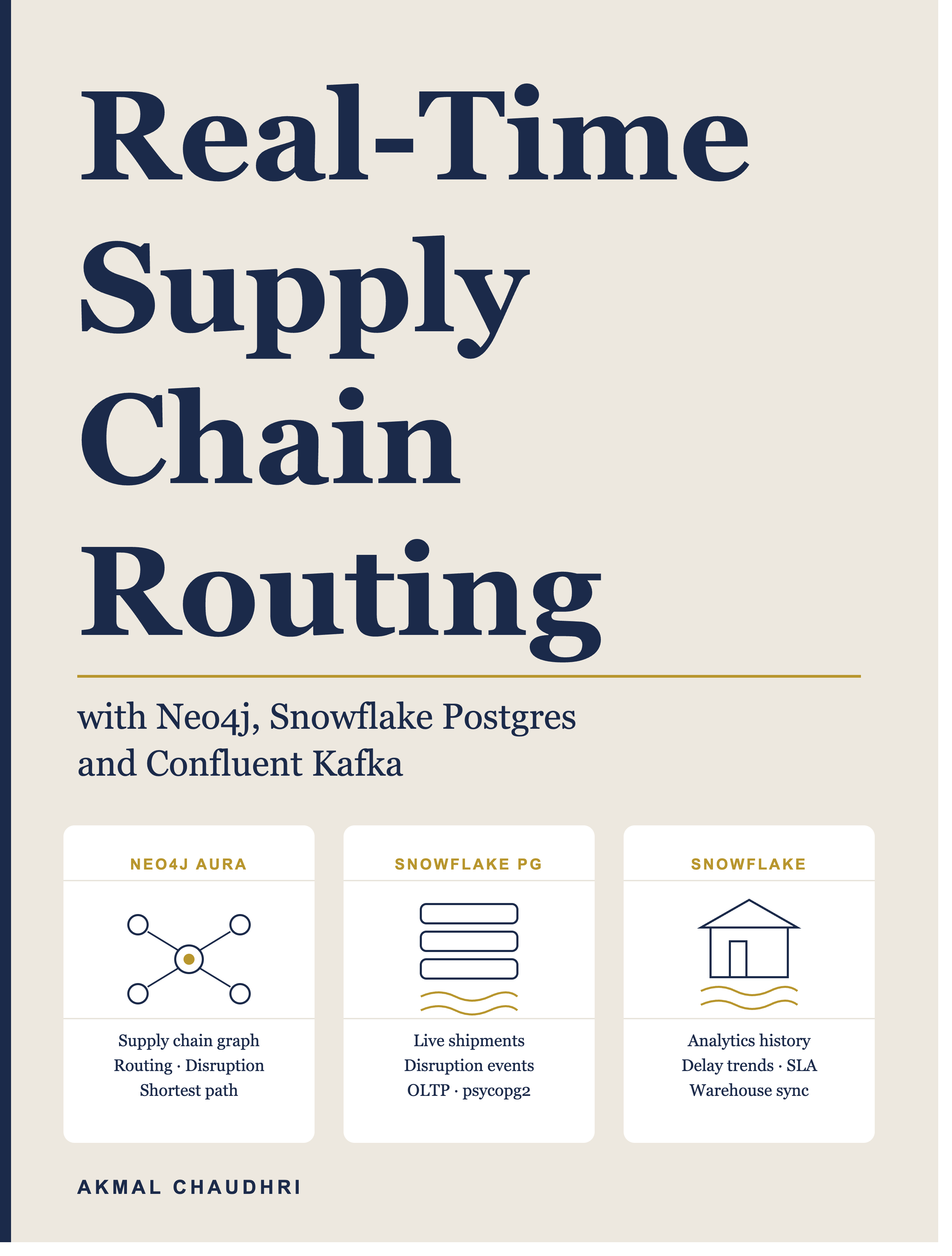
Cover

License

Publication Information

First published: September 2026

The latest version of this book, together with updates, errata and additional resources, is available at:

realtime-supply-chain.github.io

Real-Time Supply Chain Routing with Neo4j, Snowflake Postgres and Confluent Kafka is licensed under the Creative Commons Attribution-NonCommercial-NoDerivatives 4.0 International License (CC BY-NC-ND 4.0).

You are free to copy and redistribute this book in any medium or format under the following conditions:

Attribution - You must give appropriate credit, provide a link to the license and indicate if changes were made.
NonCommercial - You may not use the material for commercial purposes.
NoDerivatives - If you remix, transform or build upon the material, you may not distribute the modified material.

The full license text is available at:

creativecommons.org/licenses/by-nc-nd/4.0

Code License

Unless otherwise stated, all code samples, notebooks, scripts and source files accompanying this book are licensed under the Apache License 2.0.

You are free to use, modify and redistribute this code, including for commercial purposes, subject to the terms of the Apache License 2.0.

The full license text is available at:

apache.org/licenses/LICENSE-2.0

This distinction means that the book’s written content is protected under the Creative Commons license, while the accompanying code remains freely available for use, modification and integration into your own projects.

Trademarks

Product names, company names and logos mentioned in this book may be trademarks or registered trademarks of their respective owners.

Their inclusion is for identification and educational purposes only and does not imply any affiliation with, sponsorship by or endorsement from the respective trademark holders. All trademarks remain the property of their respective owners.

Disclaimer

The information in this book, including all code samples, scripts and notebooks, is provided “as is” without warranty of any kind, express or implied.

The author makes no representations or warranties regarding the accuracy, completeness, reliability or suitability of the information contained herein for any particular purpose.

Examples are provided solely to illustrate technical concepts, patterns and software architectures.

Readers are responsible for independently validating all code, configurations and recommendations before using them in production environments.

To the fullest extent permitted by law, the author shall not be liable for any direct, indirect, incidental, special, consequential or other damages arising from the use of or inability to use, the information, code or techniques described in this book.

About the Author

Akmal Chaudhri is a technical leader, educator and author with extensive experience in databases, AI and developer relations. He specializes in technical writing, developer education and community building, helping engineers and organizations understand and adopt complex technologies through clear, practical and engaging content. He is a frequent international speaker, a published author and a contributor to industry discussions on data platforms, AI and software development.

Today, Akmal works in developer education at Neo4j, where he focuses on technical content, workshops and community initiatives. While his professional role has evolved, this book represents an independent exploration of various data platforms.

Based in the United Kingdom, Akmal continues to work at the intersection of databases, AI and developer tooling, helping developers build modern data-driven applications.

For book updates, code samples and additional resources, visit the Book website.

To connect professionally or follow his latest work, visit LinkedIn.

Real-Time Supply Chain Routing with Neo4j, Snowflake Postgres and Confluent Kafka

This book builds a real-time supply chain operations dashboard using three database systems:

Neo4j Aura for the supply chain graph.
Snowflake Postgres for live shipment records.
Snowflake for historical analytics.

A simulated supply chain generates shipment events that flow through a Confluent Cloud Kafka topic in real time. Warehouse disruptions are injected automatically, triggering live rerouting through the Neo4j graph. Two Streamlit dashboards show live operations and analytics.

How the Code Is Organized

All runnable code lives in the code/ directory.

Notebooks are numbered to match the chapters – 02_neo4j_supply_chain.ipynb corresponds to Chapter 2, and so on.

Chapter 1: Architecture and Setup

What We’re Building

Real-time supply chain routing sits at the intersection of three distinct data problems:

Graph problem – which route connects a supplier to a retailer through active warehouses, and what’s the best alternative when one goes offline?
Operational problem – what’s the current status of each shipment and which ones have been rerouted?
Analytical problem – which warehouses are causing the most delays, which suppliers have the highest delay rates and where are SLA breaches concentrated?

Each of those problems has a natural home in a different kind of database. That’s the core idea behind this book. We’re not going to use one database and make it do everything. We’re going to use three and let each one do what it does best.

The system we’ll build is a real-time supply chain dashboard with 20 suppliers, 12 warehouses, 10 distribution centers and 30 retailers. A simulator generates shipment events that flow through a Confluent Cloud Kafka topic. Warehouse disruptions are injected automatically and the Neo4j graph finds alternative routes in real time. Two Streamlit dashboards show live operations and historical analytics.

The Three-System Architecture

The architecture has three layers, each serving a different purpose.

Neo4j Aura is the graph layer. It holds the supply chain network – suppliers, warehouses, distribution centers and retailers connected by shipping relationships. Aura answers the questions that a relational database handles with difficulty:

What’s the shortest path from a supplier to a retailer through active warehouses?
When a warehouse goes offline, which alternative route avoids it?
Which nodes are the most connected hubs of the network?

The variable-length path queries and inline filtering that Cypher provides make disruption routing fast and clean.

Snowflake Postgres is the operational layer. It’s a fully managed Postgres database, hosted inside Snowflake, that accepts the high-frequency shipment writes from our Kafka consumer. Every event consumed from the shipment-events topic is written here in real time. Snowflake Postgres handles this with standard psycopg2 connectivity. The shipments and disruption_events tables give the live operations dashboard everything it needs.

Snowflake is the analytics layer. Shipment data flows from Snowflake Postgres into a shipment_history table using an incremental sync pattern. We run aggregations here – delay trends over time, warehouse health scores, supplier delay rates and SLA breach analysis. The analytics Streamlit app syncs and queries this layer on every refresh.

The relationship between these systems is as follows:

Aura is where the structure lives – the supply chain graph that neither Snowflake Postgres nor Snowflake knows anything about.
Snowflake Postgres is where data are written, in real time, by the Kafka consumer.
Snowflake is where we analyze the history that Snowflake Postgres accumulates.

Each system has a clear role and none of the roles overlap.

What Aura Adds

A natural question is: what does Aura add? We already have a Postgres database. Can’t we just store supply chain relationships there too? We could store them there. But querying them could be difficult. Finding the shortest path from a supplier to a retailer that avoids a disrupted warehouse requires traversing a graph – following edges from node to node, filtering out inactive nodes mid-path. In SQL this means recursive CTEs with exclusion logic, which become unwieldy fast. In Cypher, Aura’s query language, it’s a concise pattern match with an inline filter:

MATCH path = (s:Supplier {id: $supplier_id})-[:SHIPS_TO*1..6]->(r:Retailer {id: $retailer_id})
WHERE NONE(n IN nodes(path) WHERE n:Warehouse AND coalesce(n.active, true) = false)
RETURN [n IN nodes(path) WHERE n:Warehouse | n.id][0] AS warehouse_id
ORDER BY length(path)
LIMIT 1

The supply chain is a graph. Suppliers ship to warehouses, warehouses ship to distribution centers, distribution centers ship to retailers. The connectivity between them is the point. Storing that as rows and columns in a relational table is possible but goes against the natural structure of the data.

What You’ll Need

To follow along you’ll need accounts and access to these services:

Neo4j Aura – the free tier is sufficient. Create an account at Get Started for Free and note your URI, username and password.
Snowflake – a free trial account gives us access to both Snowflake Postgres and the Snowflake warehouse. Create an account at Try Snowflake for Free. Create a Snowflake Postgres instance and a warehouse before running the notebooks.
Confluent Cloud – a free trial account is sufficient. Create an account at Get Started with Confluent and create a cluster with a topic named shipment-events.
Python – we’ll use Python 3.12 throughout. The notebooks run in a local Jupyter environment. A virtual environment is highly recommended. For example:

python3 -m venv ~/supply-chain-env
source ~/supply-chain-env/bin/activate

All dependencies are installed using %pip install cells at the top of each notebook, with pinned versions for stability.

Environment Variables

Credentials are passed to notebooks and the Streamlit applications using environment variables. Set these before starting Jupyter:

# Neo4j Aura
export NEO4J_URI="neo4j+s://xxxx.databases.neo4j.io"
export NEO4J_USERNAME="your-username"
export NEO4J_PASSWORD="your-password"

# Snowflake Postgres
export SNOWFLAKE_PG_HOST="your-instance.eu-west-2.aws.postgres.snowflake.app"
export SNOWFLAKE_PG_USER="snowflake_admin"
export SNOWFLAKE_PG_PASSWORD="your-password"
export SNOWFLAKE_PG_DBNAME="postgres"

# Snowflake warehouse
export SNOWFLAKE_ACCOUNT="your-account-identifier"
export SNOWFLAKE_USER="your-username"
export SNOWFLAKE_PASSWORD="your-password"
export SNOWFLAKE_DATABASE="SUPPLY_CHAIN"
export SNOWFLAKE_SCHEMA="PUBLIC"
export SNOWFLAKE_WAREHOUSE="SUPPLY_CHAIN_WH"

# Confluent Cloud
export CONFLUENT_BOOTSTRAP_SERVERS="your-cluster.confluent.cloud:9092"
export CONFLUENT_API_KEY="your-api-key"
export CONFLUENT_API_SECRET="your-api-secret"

Chapter Overview

Here’s what each chapter covers:

Chapter 2: The Supply Chain Graph walks through building the supply chain network in Neo4j Aura – 20 suppliers, 12 warehouses, 10 distribution centers and 30 retailers connected by shipping relationships. We’ll cover the Cypher queries that make routing and disruption handling efficient, including shortest path and variable-length path queries.

Chapter 3: The Operational Layer sets up Snowflake Postgres as the operational store for live shipment records. We’ll cover the table design, indexes and the disruption_events table that records every warehouse disruption and restore event.

Chapter 4: The Analytics Layer sets up the Snowflake warehouse as the analytics layer for historical shipment data. We’ll cover the shipment_history table, the incremental sync pattern that keeps it current and how the analytics app uses it on every refresh.

Chapter 5: The Simulator writes a Kafka producer and consumer that generate synthetic shipment events and write them to both Neo4j and Snowflake Postgres in real time. Warehouse disruptions fire randomly, triggering live rerouting through the Neo4j graph.

Chapter 6: The Streamlit Apps covers the two Streamlit dashboards – the live operations dashboard (app.py) showing current shipment status, active disruptions and rerouted shipments and the analytics dashboard (analytics_app.py) showing delay trends, warehouse health, shipment flow and supplier performance. There is also an optional analytics notebook for deeper one-off analysis.

Chapter 7: Bringing It All Together explains how the three systems work as a unit, covers the order of operations for running the full stack end-to-end and suggests directions for taking the project further.

Let’s start by building the supply chain graph.

Chapter 2: The Supply Chain Graph

What We Need From the Graph

The supply chain graph is the foundation of the routing system. Without it, we can’t find paths from suppliers to retailers, identify alternative routes when a warehouse goes offline or understand the connectivity of the network. Everything the simulator and the Streamlit application do around routing depends on having an accurate, connected graph of the supply chain.

We specifically need:

Every supplier, warehouse, distribution center and retailer as a node.
Every shipping relationship as a directed edge.
A way to find paths from any supplier to any retailer through active warehouses.
A way to exclude disrupted warehouses from routing without changing the graph structure.

The Aura Graph Model

The supply chain maps naturally to Aura’s property graph model. Here’s what we’re storing:

(:Supplier {id, name, location})
    -[:SHIPS_TO]->
(:Warehouse {id, name, location, active})
    -[:SHIPS_TO]->
(:DistributionCenter {id, name, location})
    -[:SHIPS_TO]->
(:Retailer {id, name, location})

Each node label represents a distinct tier of the supply chain. The active property on Warehouse nodes is the key to disruption routing – setting it to false marks a warehouse as offline without deleting it from the graph. The routing query filters out inactive warehouses mid-path using a WHERE NONE() clause.

Shipment events from the Kafka consumer are stored as Shipment nodes with relationships back to the supplier, warehouse, distribution center and retailer involved:

(:Supplier)-[:HAS_SHIPMENT]->(:Shipment)-[:VIA_WAREHOUSE]->(:Warehouse)
(:Shipment)-[:VIA_DIST_CENTER]->(:DistributionCenter)
(:Shipment)-[:DESTINED_FOR]->(:Retailer)

Building the Network

The supply chain is generated synthetically using a fixed random seed, which guarantees that the same node IDs appear in every notebook and in the simulator. The node counts are:

20 suppliers: S000 to S019
12 warehouses: W000 to W011
10 distribution centers: DC000 to DC009
30 retailers: R000 to R029

Each supplier is connected to a random subset of warehouses, each warehouse to a random subset of distribution centers and each distribution center to a random subset of retailers. The connections are sparse enough to make routing non-trivial but dense enough to ensure there’s always an alternative path when a warehouse goes offline.

Loading Into Aura

We load nodes and relationships in separate passes using MERGE to make the operation idempotent. Running the notebook twice or more won’t create duplicate nodes.

Nodes. Each tier is loaded with a uniqueness constraint on id:

UNWIND $rows AS row
MERGE (s:Supplier {id: row.id})
SET s.name     = row.name,
    s.location = row.location

The same pattern applies for Warehouse, DistributionCenter and Retailer nodes. Warehouses get an additional active property, defaulting to true.

Relationships. Each shipping connection becomes a SHIPS_TO relationship:

UNWIND $rows AS row
MATCH (a {id: row.from_id})
MATCH (b {id: row.to_id})
MERGE (a)-[:SHIPS_TO]->(b)

We load in batches of 500 rows at a time.

Clearing Before Reload

We clear the graph before each run to keep the notebook idempotent:

MATCH (n)
CALL (n) { DETACH DELETE n } IN TRANSACTIONS OF 1000 ROWS

Indexes

We create indexes on id for all four node labels before loading and an index on Shipment.status for the queries used by the analytics notebook:

CREATE INDEX supplier_id     IF NOT EXISTS FOR (n:Supplier)           ON (n.id)
CREATE INDEX warehouse_id    IF NOT EXISTS FOR (n:Warehouse)          ON (n.id)
CREATE INDEX dist_center_id  IF NOT EXISTS FOR (n:DistributionCenter) ON (n.id)
CREATE INDEX retailer_id     IF NOT EXISTS FOR (n:Retailer)           ON (n.id)
CREATE INDEX shipment_status IF NOT EXISTS FOR (n:Shipment)           ON (n.status)

Routing Queries

With the graph in place, two routing queries drive the rest of the system.

Normal routing – finding the path from a supplier to a retailer:

MATCH path = shortestPath(
    (s:Supplier {id: $supplier_id})-[:SHIPS_TO*]->(r:Retailer {id: $retailer_id})
)
RETURN [n IN nodes(path) WHERE n:Warehouse | n.id][0] AS warehouse_id

Disruption routing – finding a path that avoids the disrupted warehouse:

MATCH path = (s:Supplier {id: $supplier_id})-[:SHIPS_TO*1..6]->(r:Retailer {id: $retailer_id})
WHERE NONE(n IN nodes(path) WHERE n:Warehouse AND coalesce(n.active, true) = false)
RETURN [n IN nodes(path) WHERE n:Warehouse | n.id][0] AS warehouse_id
ORDER BY length(path)
LIMIT 1

The disruption query uses a variable-length path rather than shortestPath() because shortestPath() can’t filter nodes mid-path. The WHERE NONE() clause checks every node in the path and rejects any path that passes through an inactive warehouse.

Disruption and Restore

Marking a warehouse as offline is a single SET operation:

MATCH (w:Warehouse {id: $warehouse_id})
SET w.active = false

Restoring it is the same in reverse:

MATCH (w:Warehouse {id: $warehouse_id})
SET w.active = true

The graph structure doesn’t change. Only the active property changes and the routing query filters accordingly on the next call.

Verifying the Result

After loading, we verify the node and relationship counts and confirm the disruption routing query returns a result for a known supplier-retailer pair:

Suppliers            : 20
Warehouses           : 12
Distribution centers : 10
Retailers            : 30
SHIPS_TO             : 172

Disruption test (S000 -> R001, W003 offline):
  Alternative route via: W001

Gotchas

shortestPath() can’t filter mid-path nodes. The normal routing query uses shortestPath(), which is fast but can’t exclude inactive nodes mid-path. The disruption routing query switches to a variable-length [:SHIPS_TO*1..6] pattern with a WHERE NONE() filter. The two queries look similar but are not interchangeable – using shortestPath() for disruption routing will return paths through the disrupted warehouse.

NONE() and three-valued logic. The WHERE NONE() clause must use coalesce(n.active, true) = false rather than n.active = false. If active is missing from a node (for example, on a DistributionCenter), n.active = false evaluates to null rather than false, which NONE() treats as a match and rejects the path incorrectly. Wrapping with coalesce() makes the check safe for all node types.

Fixed random seed. The supply chain topology is generated with RANDOM_SEED = 42. Every notebook and the simulator use the same seed, which guarantees that node IDs match across the system. Changing the seed will produce a different graph and break the cross-notebook consistency.

Chapter 3: The Operational Layer

What We Need From the Operational Layer

The supply chain graph in Chapter 2 gives us the structure – the nodes and relationships that define how suppliers connect to retailers through warehouses and distribution centers. What it doesn’t give us is a place to write live shipment events as they arrive from Kafka.

We need an operational store that can:

Accept high-frequency writes from the Kafka consumer in real time.
Record the current status of every shipment.
Flag rerouted shipments and store the alternative warehouse used.
Log every warehouse disruption and restore event with a timestamp.
Serve the live operations Streamlit dashboard with fast reads.

Snowflake Postgres is that store. It’s a fully managed Postgres database hosted inside Snowflake that accepts connections from standard psycopg2 clients. The connection pattern is identical to any other managed Postgres service.

The Schema

Two tables hold all the operational data.

shipments is the primary table. Every event consumed from the shipment-events Kafka topic is written here. If a shipment is rerouted, the rerouted flag is set to true and the alternative warehouse is recorded in alt_warehouse_id:

CREATE TABLE shipments (
    shipment_id      TEXT PRIMARY KEY,
    supplier_id      TEXT        NOT NULL,
    warehouse_id     TEXT        NOT NULL,
    dist_center_id   TEXT        NOT NULL,
    retailer_id      TEXT        NOT NULL,
    status           TEXT        NOT NULL,
    delay_minutes    INTEGER     NOT NULL DEFAULT 0,
    rerouted         BOOLEAN     NOT NULL DEFAULT FALSE,
    alt_warehouse_id TEXT,
    recorded_at      TIMESTAMPTZ NOT NULL DEFAULT NOW()
)

disruption_events records every warehouse disruption and restore event. The simulator writes a row each time a warehouse goes offline and again when it comes back online. The live operations dashboard reads this table to determine the current phase and display the disruption banner:

CREATE TABLE disruption_events (
    id            SERIAL PRIMARY KEY,
    warehouse_id  TEXT        NOT NULL,
    event_type    TEXT        NOT NULL,
    recorded_at   TIMESTAMPTZ NOT NULL DEFAULT NOW()
)

The event_type column holds either disrupted or restored. The most recent row tells the dashboard which phase the system is currently in.

Both tables are created using a loop to keep the notebook concise:

tables = {
    "shipments":         "CREATE TABLE shipments ...",
    "disruption_events": "CREATE TABLE disruption_events ...",
}

for name, ddl in tables.items():
    cursor.execute(f"DROP TABLE IF EXISTS {name}")
    cursor.execute(ddl)
    print(f"Table {name} created.")

Indexes

We create indexes on the columns most commonly used in dashboard queries:

CREATE INDEX idx_shipments_status      ON shipments (status);
CREATE INDEX idx_shipments_warehouse   ON shipments (warehouse_id);
CREATE INDEX idx_shipments_recorded_at ON shipments (recorded_at DESC);
CREATE INDEX idx_shipments_rerouted    ON shipments (rerouted);

The status index speeds up the per-status counts shown in the metric tiles. The warehouse_id index speeds up the delayed-by-warehouse bar chart. The recorded_at index speeds up the incremental sync used by the analytics layer in Chapter 4. The rerouted index speeds up the rerouted shipments table.

Role Setup

We create a dedicated application role with the minimum permissions needed to read and write both tables. No superuser privileges are granted. The DO block skips creation cleanly if the role already exists, making the cell safe to re-run:

DO $$
BEGIN
    IF NOT EXISTS (SELECT FROM pg_roles WHERE rolname = 'supply_chain_app') THEN
        CREATE ROLE supply_chain_app LOGIN PASSWORD 'change-me-in-production';
    END IF;
END
$$;

GRANT USAGE ON SCHEMA public TO supply_chain_app;
GRANT SELECT, INSERT, UPDATE, DELETE ON TABLE shipments TO supply_chain_app;
GRANT SELECT, INSERT, UPDATE, DELETE ON TABLE disruption_events TO supply_chain_app;

The ALTER DEFAULT PRIVILEGES statement ensures any future tables in the schema are also accessible to the role without an additional grant.

Connecting From Python

The connection pattern is standard psycopg2. SSL is required for all Snowflake Postgres connections:

conn = psycopg2.connect(
    host     = SNOWFLAKE_PG_HOST,
    user     = SNOWFLAKE_PG_USER,
    password = SNOWFLAKE_PG_PASSWORD,
    dbname   = SNOWFLAKE_PG_DBNAME,
    sslmode  = "require",
    port     = 5432,
)
conn.autocommit = True

autocommit = True is set for DDL statements. The simulator uses the same connection pattern and relies on autocommit for the high-frequency event writes.

Verifying the Result

After creating both tables and indexes, we confirm the column definitions and index names match expectations:

Table: shipments
  Column               Type                     Nullable   Default
  ----------------------------------------------------------------------
  shipment_id          text                     NO
  supplier_id          text                     NO
  warehouse_id         text                     NO
  dist_center_id       text                     NO
  retailer_id          text                     NO
  status               text                     NO
  delay_minutes        integer                  NO         0
  rerouted             boolean                  NO         false
  alt_warehouse_id     text                     YES
  recorded_at          timestamp with time zone NO         now()

Table: disruption_events
  Column               Type                     Nullable   Default
  ----------------------------------------------------------------------
  id                   integer                  NO
  warehouse_id         text                     NO
  event_type           text                     NO
  recorded_at          timestamp with time zone NO         now()

Indexes (shipments):
  idx_shipments_recorded_at
  idx_shipments_rerouted
  idx_shipments_status
  idx_shipments_warehouse
  shipments_pkey

What the Simulator Writes

The simulator writes to both tables on every lifecycle event. For shipment events, it uses ON CONFLICT DO UPDATE to handle rerouted shipments correctly – if a shipment arrives that was initially routed through a warehouse that then went offline, the update overwrites the routing fields rather than creating a duplicate row:

INSERT INTO shipments (...)
VALUES (...)
ON CONFLICT (shipment_id) DO UPDATE
    SET rerouted         = EXCLUDED.rerouted,
        alt_warehouse_id = EXCLUDED.alt_warehouse_id,
        status           = EXCLUDED.status

For disruption events, it’s a plain insert each time a warehouse changes state:

INSERT INTO disruption_events (warehouse_id, event_type)
VALUES (%s, %s)

The recorded_at timestamp is set by the database using DEFAULT NOW(), which ensures the timestamp reflects when the event landed in Postgres rather than when it was generated by the simulator.

Gotchas

ON CONFLICT DO UPDATE not DO NOTHING. Using DO NOTHING for shipment inserts means rerouted events are silently dropped when the original shipment row already exists. The rerouted flag and alternative warehouse ID never get written. Always use DO UPDATE and explicitly set the rerouting columns.

disruption_events grant must be explicit. The ALTER DEFAULT PRIVILEGES statement only covers tables created after it runs. Since disruption_events is created before the default privileges are set, it needs its own explicit GRANT statement. Relying on default privileges alone leaves the table inaccessible to the application role.

Chapter 4: The Analytics Layer

What the Analytics Layer Does

Snowflake Postgres in Chapter 3 gives us a fast operational store for live shipment events. But it’s optimized for writes and point reads, not for the heavier aggregation queries that answer questions like “which warehouses are causing the most delays over time?” or “how has the average delay changed across the last hour?”

For those questions we need an analytics layer – somewhere to accumulate historical data and run aggregations without affecting the operational store. The Snowflake warehouse is that layer.

The analytics layer needs to:

Store a full history of shipment events as they accumulate over a run.
Stay current with new events arriving from Snowflake Postgres.
Serve the analytics Streamlit dashboard with the five charts it displays on every refresh.
Handle heavier aggregation queries efficiently without impacting live operations.

The Incremental Sync Pattern

Rather than writing directly to the Snowflake warehouse from the simulator, we use an incremental sync pattern. The analytics app (and the notebook in Chapter 6) reads new rows from the shipments table in Snowflake Postgres and appends them to shipment_history in the Snowflake warehouse.

The sync tracks a watermark – the MAX(recorded_at) already in shipment_history. On each sync call, it pulls only rows newer than that watermark and appends them:

def sync_to_warehouse(sf_cur):
    sf_cur.execute("SELECT MAX(recorded_at) FROM shipment_history")
    last_synced_at = sf_cur.fetchone()[0] or datetime(1970, 1, 1, tzinfo=timezone.utc)

    pg_cur.execute("""
        SELECT * FROM shipments
        WHERE recorded_at > %s
        ORDER BY recorded_at
    """, (last_synced_at,))

    rows = pg_cur.fetchall()
    # batch insert into shipment_history ...
    return len(rows)

This pattern is the same one used by the analytics Streamlit app on every 30-second refresh. Running it in the notebook here confirms the mechanism works before the Kafka layer is running.

The first run will find no rows since the simulator hasn’t started yet. That’s expected.

The Shipment History Table

The shipment_history table mirrors the shipments table in Snowflake Postgres but is designed for analytics rather than transactions. It has no primary key constraint since it’s append-only and adds a synced_at column recording when each row was pulled from Snowflake Postgres:

CREATE TABLE shipment_history (
    shipment_id      TEXT,
    supplier_id      TEXT,
    warehouse_id     TEXT,
    dist_center_id   TEXT,
    retailer_id      TEXT,
    status           TEXT,
    delay_minutes    INTEGER,
    rerouted         BOOLEAN,
    alt_warehouse_id TEXT,
    recorded_at      TIMESTAMP_TZ,
    synced_at        TIMESTAMP_TZ
)

The table is dropped and recreated on each notebook run, so the notebook is safe to re-run from the start during development. In the analytics Streamlit app the table persists across refreshes and the incremental sync keeps it current.

Connecting to Snowflake

We use the snowflake-connector-python library to connect to the Snowflake warehouse. The account identifier is the part of the Snowflake URL:

sf = snowflake.connector.connect(
    account  = SNOWFLAKE_ACCOUNT,
    user     = SNOWFLAKE_USER,
    password = SNOWFLAKE_PASSWORD,
)
sf_cursor = sf.cursor()
sf_cursor.execute(f"USE DATABASE {SNOWFLAKE_DATABASE}")
sf_cursor.execute(f"USE SCHEMA {SNOWFLAKE_SCHEMA}")
sf_cursor.execute(f"USE WAREHOUSE {SNOWFLAKE_WAREHOUSE}")

The Compute Warehouse

The Snowflake compute warehouse runs the analytics queries. We use an X-SMALL warehouse with auto-suspend and auto-resume to keep costs low. It spins up when a query arrives and suspends automatically after 60 seconds of inactivity:

CREATE WAREHOUSE IF NOT EXISTS SUPPLY_CHAIN_WH
WITH WAREHOUSE_SIZE      = 'X-SMALL'
     AUTO_SUSPEND        = 60
     AUTO_RESUME         = TRUE
     INITIALLY_SUSPENDED = TRUE

INITIALLY_SUSPENDED = TRUE means the warehouse doesn’t consume credits until the first query runs.

Batch Inserts

The sync function inserts rows in batches of 500 using executemany with %s placeholders:

BATCH_SIZE = 500
for i in range(0, len(rows), BATCH_SIZE):
    batch = rows[i:i + BATCH_SIZE]
    placeholders = ", ".join(["%s"] * 11)
    sf_cur.executemany(
        f"INSERT INTO shipment_history VALUES ({placeholders})",
        values_list,
    )

Timestamps are converted to strings before insertion to ensure the Snowflake connector handles them correctly.

Verifying the Result

After creating the table and running the initial sync, we confirm the column definitions match expectations and check the row count:

Table: shipment_history
  Column               Type
  ----------------------------------------
  SHIPMENT_ID          TEXT
  SUPPLIER_ID          TEXT
  WAREHOUSE_ID         TEXT
  DIST_CENTER_ID       TEXT
  RETAILER_ID          TEXT
  STATUS               TEXT
  DELAY_MINUTES        NUMBER
  REROUTED             BOOLEAN
  ALT_WAREHOUSE_ID     TEXT
  RECORDED_AT          TIMESTAMP_TZ
  SYNCED_AT            TIMESTAMP_TZ

Row count: 0

Zero rows is correct at this stage – the simulator hasn’t run yet.

Gotchas

mogrify behaves differently on the Snowflake connector than on psycopg2. The Snowflake connector’s mogrify may not correctly escape all Python types, particularly timestamps and booleans. Use executemany with %s placeholders instead. This is the pattern used throughout the analytics notebook and the Streamlit app.

Timestamp binding. Convert datetime objects to strings before inserting into Snowflake. The connector doesn’t always handle timezone-aware datetime objects correctly. Wrapping with str(v) if hasattr(v, 'isoformat') else v ensures safe binding for all timestamp columns.

CREATE TABLE IF NOT EXISTS in the analytics app. The analytics notebook drops and recreates shipment_history on each run. The analytics Streamlit app doesn’t – it creates the table only if it doesn’t already exist, then appends to it incrementally. Ensure the notebook and the app aren’t run simultaneously, as the notebook’s DROP TABLE will delete data the app has already accumulated.

Chapter 5: The Simulator

What the Simulator Does

The simulator generates synthetic shipment events, publishes them to a Confluent Cloud Kafka topic and consumes them back in real time. For each consumed event, it writes the shipment to both Neo4j and Snowflake Postgres – and if the shipment passes through a warehouse that’s currently offline, it reroutes it through an alternative warehouse found via the Neo4j graph.

The simulator has four responsibilities:

Publish synthetic shipment events to the shipment-events Kafka topic.
Consume those events from the same topic.
Inject warehouse disruptions at random intervals and restore them after a random duration.
Write every event to Neo4j and Snowflake Postgres, with rerouting applied where needed.

It runs directly in a Jupyter notebook cell. The loop stops on keyboard interrupt or automatically after MAX_RUNTIME_SECONDS.

The Kafka Producer and Consumer

The simulator uses confluent-kafka for both producing and consuming events. The producer publishes one event per iteration of the loop. The consumer reads one event back before writing to the databases. This tight produce-consume loop ensures that what gets written to Neo4j and Snowflake Postgres is exactly what landed in Kafka – the same event, with the same timestamp.

Both producer and consumer authenticate with SASL/SSL:

producer = Producer({
    "bootstrap.servers": CONFLUENT_BOOTSTRAP_SERVERS,
    "security.protocol": "SASL_SSL",
    "sasl.mechanisms":   "PLAIN",
    "sasl.username":     CONFLUENT_API_KEY,
    "sasl.password":     CONFLUENT_API_SECRET,
})

The consumer uses a fixed group.id and auto.offset.reset = "earliest" to ensure it picks up from the beginning of the topic on each run.

Generating Shipment Events

Each shipment event is generated with a fixed random seed, which makes the sequence reproducible:

rng  = np.random.default_rng(RANDOM_SEED)

def make_shipment_event():
    status = str(rng.choice(STATUSES, p=STATUS_WEIGHTS))
    return {
        "shipment_id":    str(uuid.uuid4()),
        "supplier_id":    str(rng.choice(SUPPLIER_IDS)),
        "warehouse_id":   str(rng.choice(WAREHOUSE_IDS)),
        "dist_center_id": str(rng.choice(DIST_CENTER_IDS)),
        "retailer_id":    str(rng.choice(RETAILER_IDS)),
        "status":         status,
        "timestamp":      time.strftime("%Y-%m-%dT%H:%M:%SZ", time.gmtime()),
        "delay_minutes":  int(rng.integers(15, 240)) if status == "delayed" else 0,
    }

Status weights are [0.25, 0.45, 0.15, 0.15] for departed, in_transit, delayed and delivered. Roughly 15% of shipments are delayed, which produces enough delay data for the analytics charts without overwhelming the status breakdown.

The Disruption Lifecycle

Warehouse disruptions fire randomly during the simulation. Two configuration parameters control the timing:

DISRUPTION_INTERVAL_MIN / DISRUPTION_INTERVAL_MAX – how many events pass between disruptions.
DISRUPTION_DURATION_MIN / DISRUPTION_DURATION_MAX – how long each disruption lasts in events.

Both the gap between disruptions and the duration of each disruption are drawn randomly from these ranges using the seeded rng. This produces a realistic pattern – disruptions are not predictable but the system is reproducible.

The first disruption always hits W003, which is the warehouse used in the Chapter 2 graph verification test. Subsequent disruptions target a randomly chosen warehouse drawn after each restore.

The lifecycle has three phases:

normal -> disrupted -> restored -> normal -> ...

Transitioning to disrupted sets the warehouse’s active property to false in Neo4j and writes a disrupted row to disruption_events in Snowflake Postgres. Transitioning to restored reverses both.

Rerouting

When the simulator is in the disrupted phase and a consumed event routes through the disrupted warehouse, it calls find_alternative_route() to ask Neo4j for a path that avoids it:

if phase == "disrupted" and consumed["warehouse_id"] == current_disruption:
    alt_warehouse_id = find_alternative_route(
        session,
        consumed["supplier_id"],
        consumed["retailer_id"],
    )

The rerouting query uses a variable-length path with a WHERE NONE() filter:

MATCH path = (s:Supplier {id: $supplier_id})-[:SHIPS_TO*1..6]->(r:Retailer {id: $retailer_id})
WHERE NONE(n IN nodes(path) WHERE n:Warehouse AND coalesce(n.active, true) = false)
RETURN [n IN nodes(path) WHERE n:Warehouse | n.id][0] AS warehouse_id
ORDER BY length(path)
LIMIT 1

If an alternative is found, alt_warehouse_id is passed to both write_to_neo4j and write_to_postgres, which record the rerouting in both systems.

Writing to Neo4j and Snowflake Postgres

Each consumed event is written to both systems before the loop advances.

Neo4j – a MERGE on shipment_id creates or updates the Shipment node and its four relationships. If the shipment was rerouted, the VIA_WAREHOUSE relationship points to the alternative warehouse rather than the original:

MERGE (sh:Shipment {shipment_id: $shipment_id})
SET sh.status        = $status,
    sh.delay_minutes = $delay_minutes,
    sh.timestamp     = $timestamp,
    sh.rerouted      = $rerouted

Neo4j writes use write_to_neo4j_with_retry(), which opens a fresh session per attempt and retries up to twice on connection failure. This handles the session timeouts that Aura enforces on long-running connections.

Snowflake Postgres – an INSERT ... ON CONFLICT DO UPDATE handles rerouted shipments correctly. If a shipment arrives that was initially routed through a warehouse that then went offline, the update overwrites the routing fields:

INSERT INTO shipments (...)
ON CONFLICT (shipment_id) DO UPDATE
    SET rerouted         = EXCLUDED.rerouted,
        alt_warehouse_id = EXCLUDED.alt_warehouse_id,
        status           = EXCLUDED.status

The Display

The simulator refreshes its output every PRINT_EVERY events, showing the current phase, the latest event and the running status breakdown:

Events processed : 1440
Phase            : DISRUPTION ACTIVE -- W003 offline
Rerouted         : 36
Refresh every    : 10

Latest event:
  !! a894fcfa... S010 -> W003 -> DC002 -> R011 [delayed]

Last reroute:
  5fbb903f... W003 -> W005

Status breakdown:
  departed     : 396
  in_transit   : 598
  delayed      : 232
  delivered    : 214

The !! prefix marks delayed events. The -> prefix marks normal events.

Runtime Limit

The simulator stops automatically after MAX_RUNTIME_SECONDS even when N_EVENTS is set to -1 for continuous operation:

start_time = time.time()
while (N_EVENTS == -1 or counter < N_EVENTS) and \
      (time.time() - start_time < MAX_RUNTIME_SECONDS):
    ...

This ensures the simulator doesn’t run indefinitely if left unattended.

Verifying the Result

A verify cell at the end of the notebook connects to Snowflake Postgres and prints a summary of both tables:

Snowflake Postgres -- shipments table by status:
  departed     : 396
  in_transit   : 598
  delayed      : 232
  delivered    : 214

  Total        : 1440
  Rerouted     : 36

Snowflake Postgres -- disruption_events:
  Warehouse    Event        Timestamp
  W003         disrupted    2026-09-07 15:18:42+00:00
  W003         restored     2026-09-07 15:21:15+00:00
  W007         disrupted    2026-09-07 15:24:03+00:00
  W007         restored     2026-09-07 15:26:44+00:00

Gotchas

Long-lived Neo4j Aura sessions time out. Aura closes idle connections after a period of inactivity, throwing SessionExpired. The fix is to open a fresh session per operation rather than holding one open for the duration of the loop. All Neo4j calls in the simulator use short-lived with neo4j_driver.session() as session: blocks and the main shipment write uses write_to_neo4j_with_retry() to handle dropped connections automatically.

Only one rerouted shipment. If the disruption window is too short relative to the event rate and the number of warehouses, very few shipments will pass through the disrupted warehouse during the disruption. Increase DISRUPTION_DURATION_MAX or decrease DISRUPTION_INTERVAL_MIN to produce more rerouting events.

ON CONFLICT DO NOTHING drops rerouted events. Using DO NOTHING for shipment inserts means rerouted events are silently dropped when the original shipment row already exists. Always use DO UPDATE and explicitly set the rerouting columns.

Tables are truncated, not dropped, at simulator startup. The shipments and disruption_events tables are owned by the Chapter 3 notebook. The simulator truncates them at startup rather than dropping and recreating them. Re-running the Chapter 3 notebook after the simulator has run will drop and recreate the tables, clearing all data.

Chapter 6: The Streamlit Apps

Two Dashboards

The system has two Streamlit dashboards. The live operations dashboard (app.py, port 8501) shows current shipment status, active disruptions, rerouted shipments and a disruption events log. The analytics dashboard (analytics_app.py, port 8502) shows status breakdown, delay trends, warehouse health, shipment flow and supplier performance, updated every 30 seconds from the Snowflake warehouse.

Run them alongside the simulator:

streamlit run app.py
streamlit run analytics_app.py --server.port 8502

The Live Operations Dashboard

Auto-Refresh

The live operations dashboard refreshes every 10 seconds. streamlit-autorefresh handles this with a single call near the top of the script:

st_autorefresh(interval=REFRESH_SECONDS * 1000)

Every 10 seconds the entire script re-runs from top to bottom, re-querying Snowflake Postgres for the latest shipment and disruption data.

Connections

All queries read from Snowflake Postgres using psycopg2. The connection is opened per query using @st.cache_data(ttl=REFRESH_SECONDS), which caches each query result for 10 seconds and avoids hammering the database on every rerun:

@st.cache_data(ttl=REFRESH_SECONDS)
def fetch_status_counts():
    with get_conn() as conn:
        with conn.cursor() as cur:
            cur.execute("""
                SELECT status, COUNT(*) AS count
                FROM shipments
                GROUP BY status
            """)
            return {row[0]: row[1] for row in cur.fetchall()}

The most prominent element on the dashboard is the disruption banner – a full-width coloured box at the top of the page. It shows green for normal operations, red when a warehouse is offline and amber immediately after a restore. After a configurable grace period (RESTORED_GRACE_SECONDS, defaulting to 60 seconds), the banner returns to green even if the last event in disruption_events was a restore.

The current phase is determined by the most recent row in disruption_events:

cur.execute("""
    SELECT event_type, warehouse_id, recorded_at
    FROM disruption_events
    ORDER BY recorded_at DESC
    LIMIT 1
""")

If the last event was disrupted, the banner is red. If it was restored and fewer than RESTORED_GRACE_SECONDS have elapsed, the banner is amber. Otherwise it’s green.

Status Metric Tiles

Four metric tiles below the banner show shipment counts for each status – departed, in_transit, delayed and delivered. Each tile uses the same color palette as the analytics dashboard’s doughnut chart for consistency across both apps.

Delayed Shipments by Warehouse

A vertical bar chart shows delayed shipment counts per warehouse, using a Reds colorscale. Warehouses with more delayed shipments appear with a deeper red fill, making the worst-performing warehouses immediately visible.

Recent Rerouted Shipments

A 10-row table shows the most recent rerouted shipments with the original warehouse, the alternative warehouse and the timestamp. This table is the most direct way to see the disruption routing in action.

Disruption Events Log

A second 10-row table at the bottom of the page shows the most recent rows from disruption_events – every warehouse disruption and restore, with timestamps. This gives an at-a-glance history of disruption activity during the current simulator run.

The Analytics Dashboard

Auto-Refresh and Sync

The analytics dashboard refreshes every 30 seconds. On each refresh it syncs new rows from shipments in Snowflake Postgres into shipment_history in the Snowflake warehouse using the incremental watermark pattern from Chapter 4:

sf_cur.execute("SELECT MAX(recorded_at) FROM shipment_history")
last_synced_at = sf_cur.fetchone()[0] or datetime(1970, 1, 1, tzinfo=timezone.utc)

Only rows newer than the watermark are pulled and appended. The first refresh after a long simulator run may sync thousands of rows; subsequent refreshes sync only the handful of rows that arrived in the last 30 seconds.

The table is created on first use with CREATE TABLE IF NOT EXISTS, so the app works whether or not the Chapter 4 notebook has been run:

sf_cur.execute("""
    CREATE TABLE IF NOT EXISTS shipment_history (...)
""")

Connections

The analytics dashboard connects to two systems:

Snowflake Postgres – for the incremental sync source.
Snowflake warehouse – for all analytics queries.

Both connections are opened at the start of each refresh and closed at the end. The Snowflake warehouse compute is an X-SMALL instance with auto-suspend, so it only consumes credits while queries are running.

Status Breakdown

The first chart is a doughnut using go.Pie with hole=0.4. The same COLOR_MAP is used throughout both apps for consistency:

COLOR_MAP = {
    "departed":   "#4C9BE8",
    "in_transit": "#2A9D8F",
    "delayed":    "#E63946",
    "delivered":  "#57CC99",
}

Delay Trends Over Time

A dual-axis line chart shows delayed shipment count per minute on the left axis and average delay duration in minutes on the right axis. The dashed line for average delay makes it easy to distinguish the two series without relying on color alone.

Warehouse Health Heatmap

A go.Heatmap shows each warehouse’s health score – the percentage of its shipments that were not delayed – on a red-to-orange-to-green colorscale. Warehouses that were disrupted during the simulator run tend to show lower health scores, which makes the heatmap a quick way to see which warehouses caused the most disruption.

Shipment Flow Sankey

A go.Sankey diagram shows the volume of shipments flowing from each supplier to each warehouse. The left nodes are suppliers (blue) and the right nodes are warehouses (teal). The width of each link is proportional to the number of shipments that took that route. Rerouting events show up as unexpected links – suppliers that don’t normally connect to a warehouse appearing with a thin link when a disruption forced their shipments there.

Top Suppliers and SLA Breach

Two horizontal bar charts sit side by side at the bottom of the dashboard. The first ranks suppliers by delay rate using a Reds colorscale. The second ranks warehouses by SLA breach rate – the percentage of shipments where delay_minutes exceeded the threshold – using an Oranges colorscale. Both charts exclude nodes with fewer than three shipments to avoid misleading results from small samples.

Gotchas

use_container_width deprecated. Streamlit deprecated use_container_width in favor of width='stretch' in recent versions. Use st.plotly_chart(fig, width='stretch') rather than use_container_width=True.

streamlit-autorefresh silent argument removed. The silent keyword argument was removed from st_autorefresh in recent versions. Use st_autorefresh(interval=N) with no additional arguments.

@st.cache_data and live data. Setting ttl too high on cached queries means the dashboard shows stale data. Set ttl to match the refresh interval so that each auto-refresh fetches fresh data from the database.

Snowflake warehouse auto-suspend. The X-SMALL compute warehouse suspends after 60 seconds of inactivity. The first query after a suspension has a cold-start delay of a few seconds while the warehouse resumes. This is normal and expected – the analytics dashboard shows a spinner while the sync and queries run.

mogrify on the Snowflake connector. The Snowflake connector’s mogrify may not correctly escape all Python types. Use executemany with %s placeholders for batch inserts into shipment_history.

Chapter 7: Bringing It All Together

The Full System

With all six chapters complete, the system looks like this:

Neo4j Aura. Holds the supply chain graph – 20 suppliers, 12 warehouses, 10 distribution centers and 30 retailers connected by shipping relationships, loaded once in Chapter 2 and updated in real time as shipments arrive. It answers graph questions: what’s the shortest path from a supplier to a retailer, which warehouse should we use when one goes offline, which nodes are the most connected hubs.
Snowflake Postgres. Holds the live operational data – every shipment event consumed from Kafka, written in real time by the simulator. It answers OLTP questions: how many shipments are currently delayed, which shipments have been rerouted, when did W003 go offline and when did it come back.
Snowflake. Holds the analytical history – shipment data synced from Snowflake Postgres into shipment_history and aggregated for trend analysis. It answers analytical questions: which suppliers have the highest delay rates, which warehouses are breaching SLA thresholds, how has delay volume changed over the last hour.

None of these systems knows about the others. Aura knows nothing about Snowflake Postgres shipment records. Snowflake Postgres knows nothing about the graph topology. Snowflake knows nothing about disruption routing. The intelligence sits in the application layer – the simulator, the Streamlit dashboards and the analytics notebook – which orchestrates queries across all three and combines the results.

Running the System

The order of operations matters. Work through the notebooks in sequence:

02_neo4j_supply_chain.ipynb – Builds the supply chain graph in Aura.
03_snowflake_postgres.ipynb – Creates the operational tables in Snowflake Postgres.
04_snowflake_warehouse.ipynb – Creates the analytics table in Snowflake.
05_simulator.ipynb – Runs the Kafka producer, consumer and disruption lifecycle.
06_analytics.ipynb – Optional, for running five analytics queries interactively.
In a terminal: streamlit run app.py.
In a second terminal: streamlit run analytics_app.py --server.port 8502.

Let the simulator run for at least 20 minutes before opening the analytics dashboard. The delay trends, warehouse health and Sankey charts need enough data to tell a meaningful story.

What Each System Does That the Others Can’t

It’s worth noting why three systems are better than one for this use case.

Why not just Aura? Neo4j Aura is purpose-built for graph traversals – exactly what the disruption routing requires. Finding an alternative path that avoids an inactive warehouse mid-route is a natural graph query. In Cypher it’s a variable-length path with a WHERE NONE() filter. In SQL it would require a recursive CTE with exclusion logic that grows in complexity with each additional hop. The graph structure also makes it easy to answer questions about connectivity – which suppliers can reach which retailers, which warehouses are the most connected hubs – that would require expensive self-joins in a relational database.

Why not just Snowflake Postgres? Snowflake Postgres is purpose-built for operational data – high-frequency writes from the Kafka consumer, transactional consistency and low-latency reads for the live operations dashboard. It handles thousands of shipment inserts per session exactly as a production Postgres instance would. Standard psycopg2 connectivity, ON CONFLICT DO UPDATE for rerouted shipments and TIMESTAMPTZ for accurate event timing all work exactly as expected.

Why not just Snowflake? Snowflake is excellent for large-scale analytics and historical queries. Aggregating delay trends by minute, computing warehouse health scores across thousands of shipments and ranking suppliers by delay rate are all queries that benefit from Snowflake’s columnar storage and parallel execution. Running these queries against the operational Snowflake Postgres table would add load to the live system and slow down the simulator’s writes.

The three-system architecture isn’t complexity for its own sake. Each system does what it’s genuinely good at and the results are combined at the application layer.

Going Further

The system as built is a working demo. Here are some directions for making it more realistic.

Real supply chain topology. The supply chain graph is generated synthetically with a fixed random seed. A natural extension is to load a real supplier-warehouse-retailer network from a CSV or an ERP system export. The MERGE-based loading pattern in Chapter 2 is already idempotent, so replacing the synthetic data with real data requires only changing the source.

Multiple disruptions simultaneously. The simulator disrupts one warehouse at a time. In reality, multiple warehouses can go offline at once – due to weather events, regional power outages or carrier failures. Extending the disruption lifecycle to track a set of disrupted warehouses rather than a single one would make the routing more challenging and the analytics more interesting.

Kafka Streams processing. The simulator currently consumes events one at a time in a tight loop. A natural production extension is to add a Kafka Streams application between the producer and the consumer that enriches events in real time – adding routing decisions, delay predictions or SLA breach flags before they land in Snowflake Postgres. This decouples the enrichment logic from the consumer and scales independently.

Real delay prediction. Delay minutes are currently drawn from a uniform random distribution. A more realistic model would use a machine learning model trained on historical delay data to predict delay duration based on supplier, warehouse, route and time of day. The delay_minutes column is already in the schema – replacing the random draw with a model prediction requires only changing the event generation function.

Snowflake Dynamic Tables. The incremental sync from Snowflake Postgres to shipment_history is handled in application code. Snowflake’s Dynamic Tables feature can automate this – defining shipment_history as a Dynamic Table that refreshes automatically whenever the source data changes. This would remove the sync code from the analytics app entirely and keep the warehouse table current without any application involvement.

Streamlit Cloud deployment. Both Streamlit apps run locally in this demo. Deploying them to Streamlit Cloud would make the dashboards accessible from any browser without running a local server. The only change required is moving credentials from environment variables to Streamlit’s secrets management.

Free Books

The SingleStore Cookbook: Recipes for Multi-Model, Machine Learning and AI Data Engineering

Read Online ↗

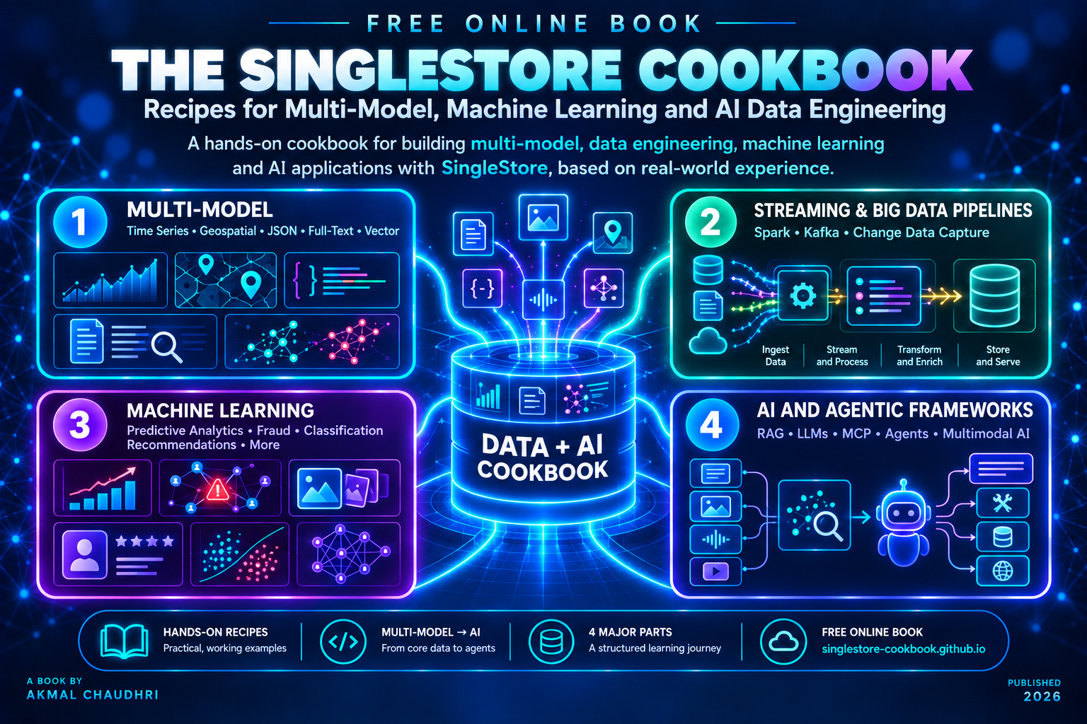
A hands-on cookbook covering SingleStore’s multi-model capabilities, from time series and geospatial data through vector search, machine learning pipelines and AI-powered applications. The recipes draw on first-hand experience building applications with the platform and are organized into four parts:

Multi-Model
Streaming and Big Data Pipelines
Machine Learning
AI and Agentic Frameworks

Seven Vector Databases in Seven Days

Read Online ↗

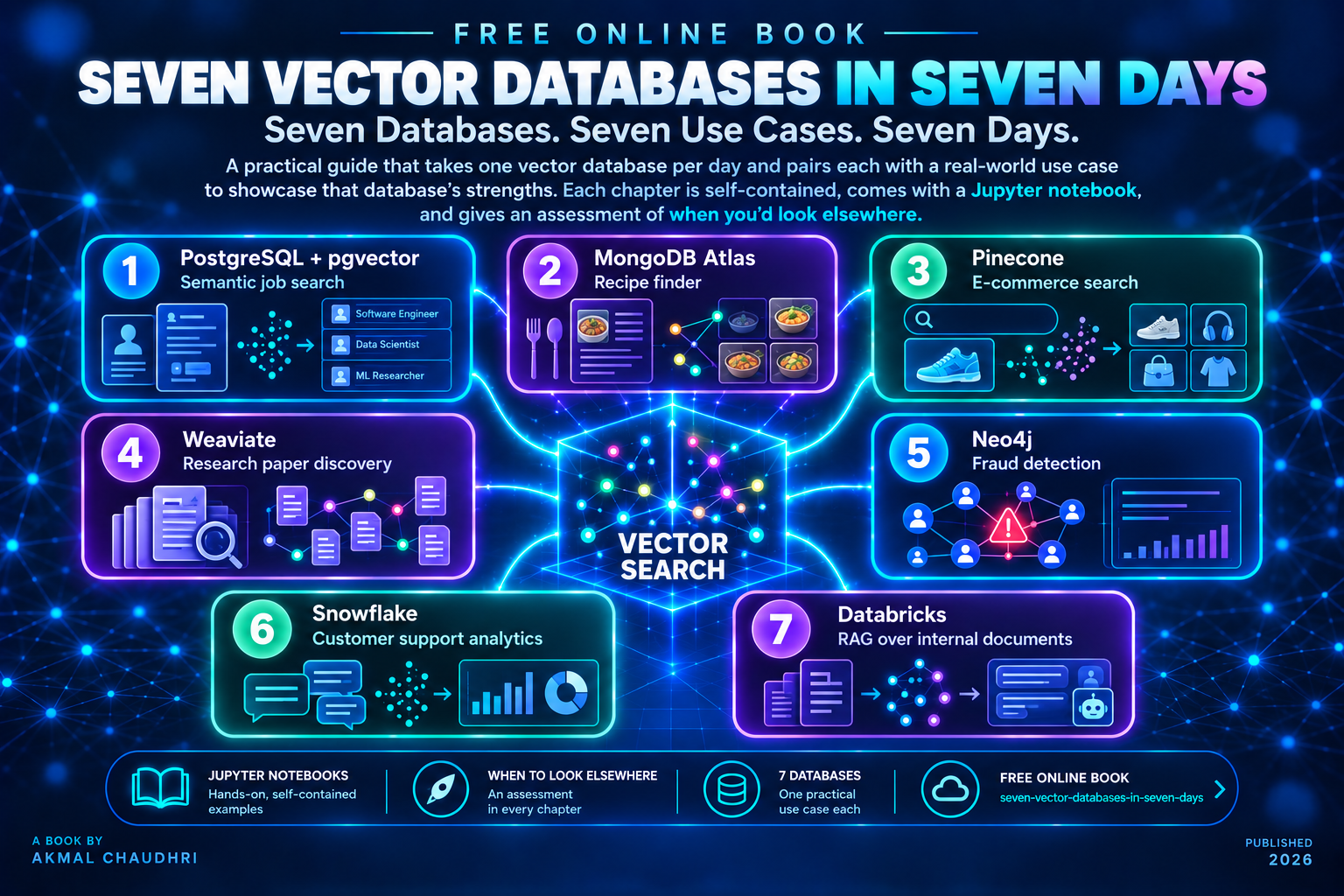
A practical guide that takes one vector database per day and pairs each with a use case chosen to showcase that database’s strengths. Databases covered:

PostgreSQL and pgvector - Semantic job search
MongoDB Atlas - Recipe finder
Pinecone - E-commerce search
Weaviate - Research paper discovery
Neo4j - Fraud detection
Snowflake - Customer support analytics
Databricks - RAG over internal documents

Each chapter is self-contained, comes with a Jupyter notebook and gives an assessment of when you’d look elsewhere.

Generative AI: A Manager’s Guide

Read Online ↗

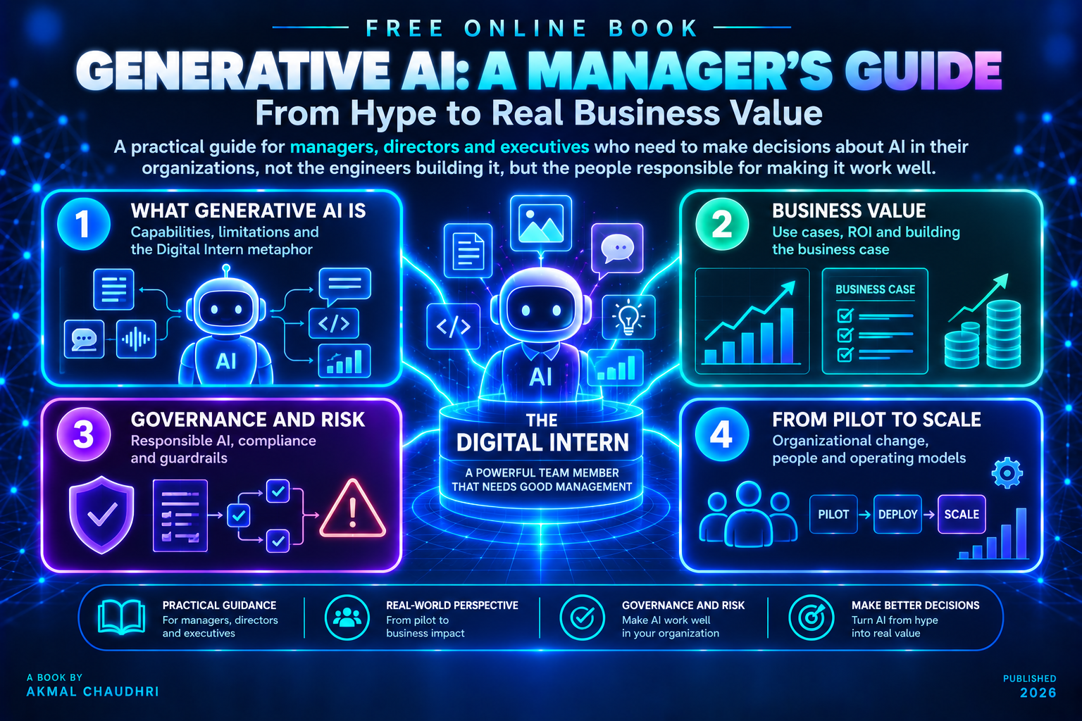
A practical guide for managers, directors and executives who need to make decisions about AI in their organizations, not the engineers building it, but the people responsible for making it work well. The book uses a single central metaphor, the Digital Intern, to frame what AI is genuinely good at, where it falls short and what managing it actually requires. It covers governance, risk, board-level accountability, business case building and the organizational change of moving from pilot to embedded capability.

Seven Ways to Do Vector Search in Python

Read Online ↗

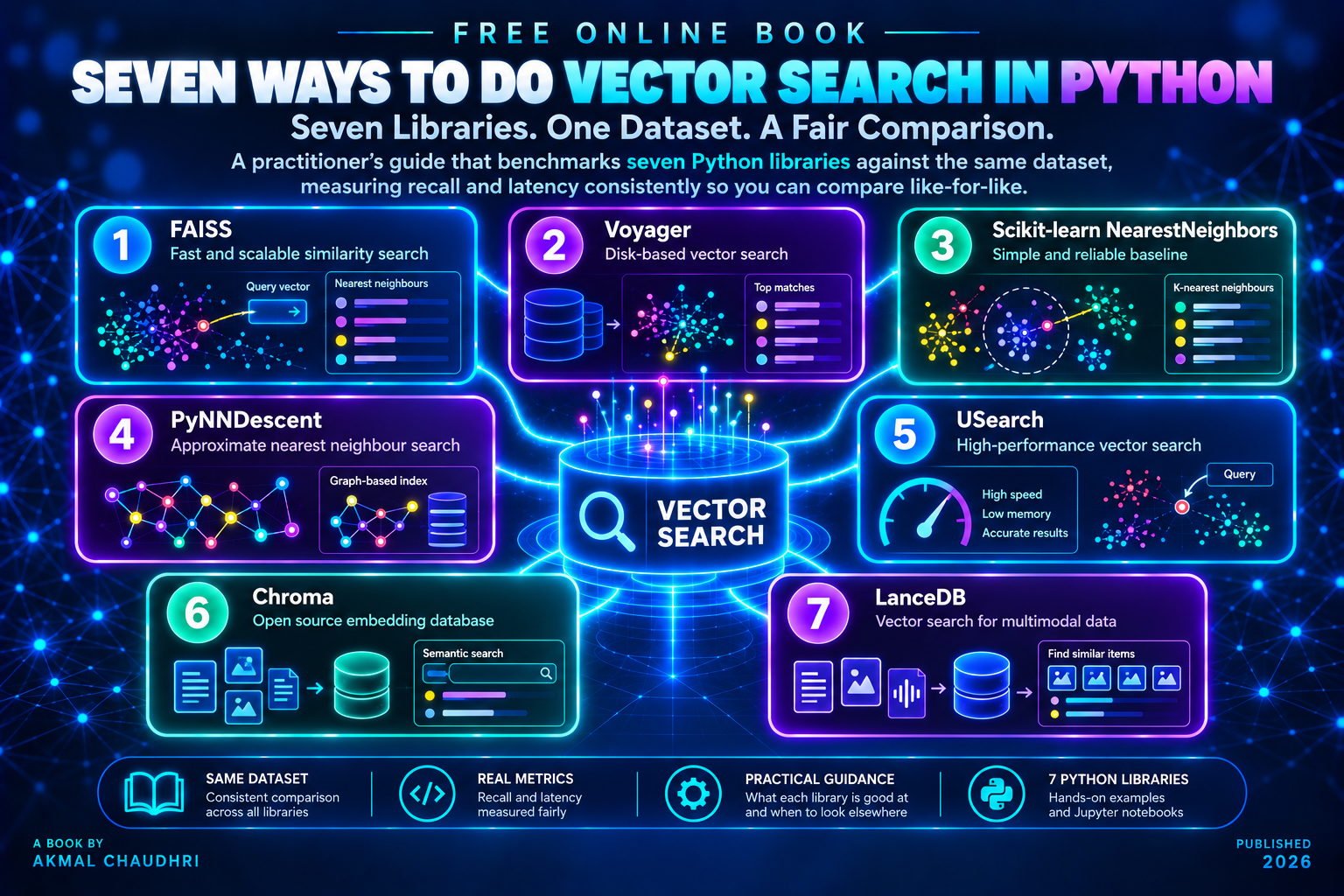
A practitioner’s guide that benchmarks seven Python libraries against the same dataset, measuring recall and latency consistently so you can compare like-for-like. Libraries covered:

FAISS
Voyager
Scikit-learn NearestNeighbors
PyNNDescent
USearch
Chroma
LanceDB

Each chapter covers one library, explains what it’s genuinely good at and when you’d reach for something else.

Real-Time Vehicle Tracking with Neo4j, Databricks Lakebase and OpenStreetMap

Read Online ↗

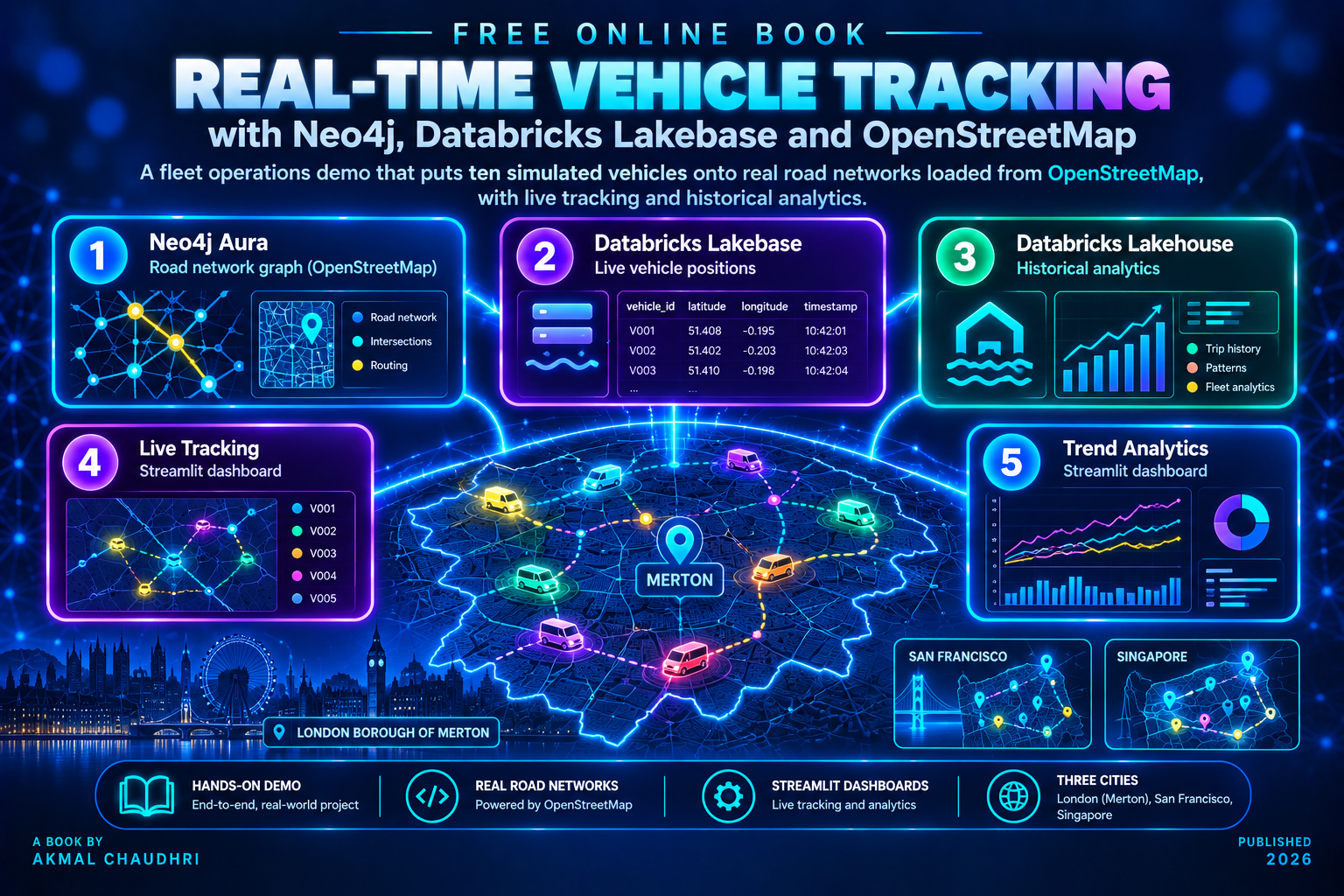
A fleet operations demo that puts ten simulated vehicles onto real road networks loaded from OpenStreetMap. The architecture:

Neo4j Aura holds the road network graph
Databricks Lakebase stores live vehicle positions
Databricks Lakehouse handles historical analytics

Two Streamlit dashboards display live positions and trend data. The primary demo uses the London Borough of Merton, with additional configurations for San Francisco and Singapore.

Real-Time Supply Chain Routing with Neo4j, Snowflake Postgres and Confluent Kafka

Read Online ↗

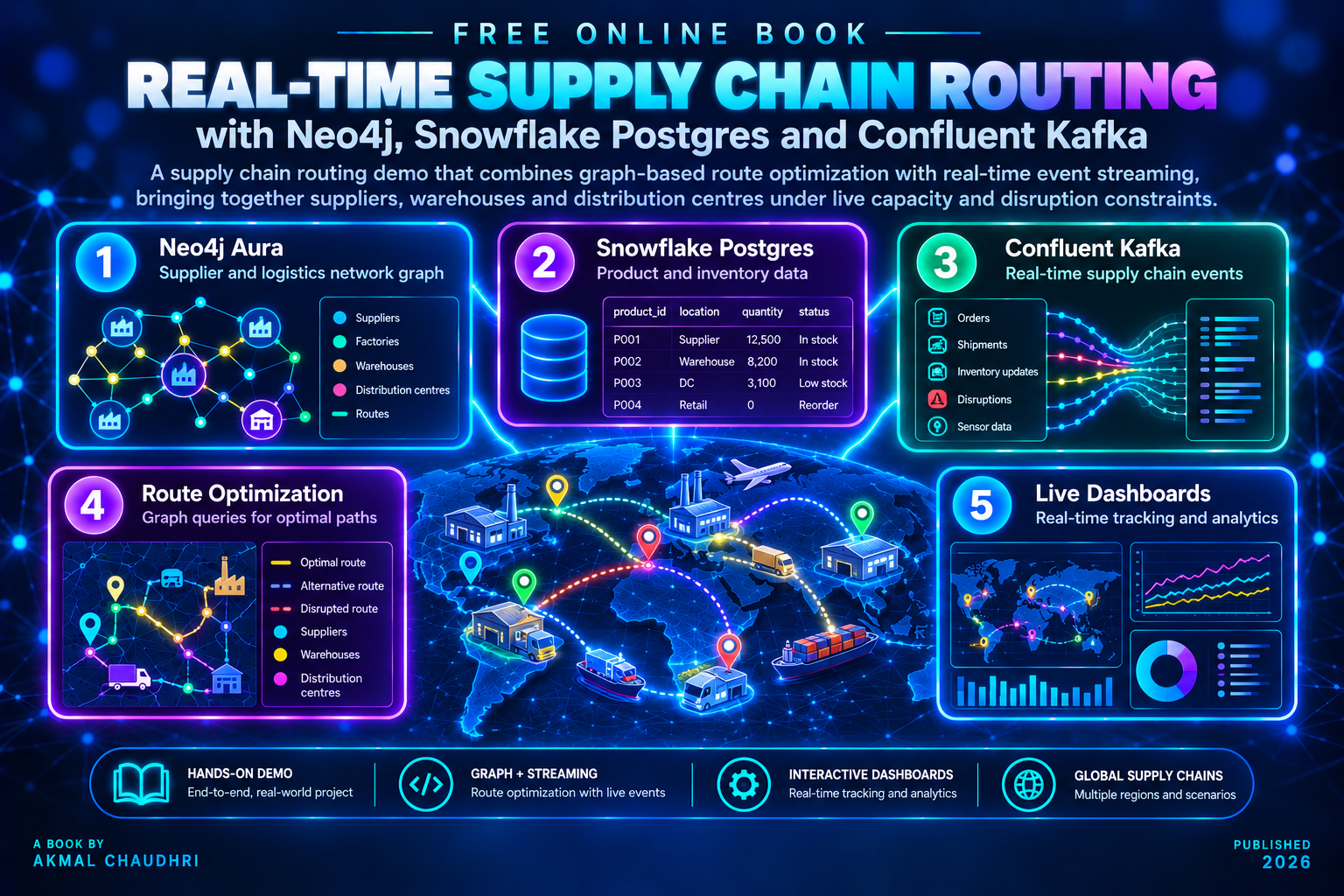
A supply chain routing demo that combines graph-based route optimization with real-time event streaming. The architecture:

Neo4j Aura holds the supplier and logistics network graph
Snowflake Postgres stores product and inventory data
Confluent Kafka streams supply chain events in real time

Route queries traverse the graph to find optimal paths between suppliers, warehouses and distribution centers under live capacity and disruption constraints.

Neo4j Beyond the Graph

Read Online ↗

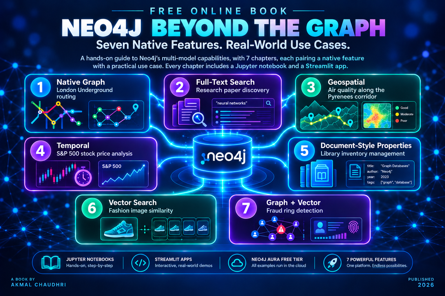
A hands-on guide to Neo4j’s multi-model capabilities, going beyond graph traversal to explore seven native features of the platform. Each chapter pairs one capability with a use case chosen to showcase it:

Native Graph - London Underground routing
Full-Text Search - Research paper discovery
Geospatial - Air quality along the Pyrenees corridor
Temporal - S&P 500 stock price analysis
Document-Style Properties - Library inventory management
Vector Search - Fashion image similarity
Graph + Vector - Fraud ring detection

Every chapter comes with a Jupyter notebook and a Streamlit application. All examples run on Neo4j Aura’s free tier.

Seven Ways to Use Jev

Read Online ↗

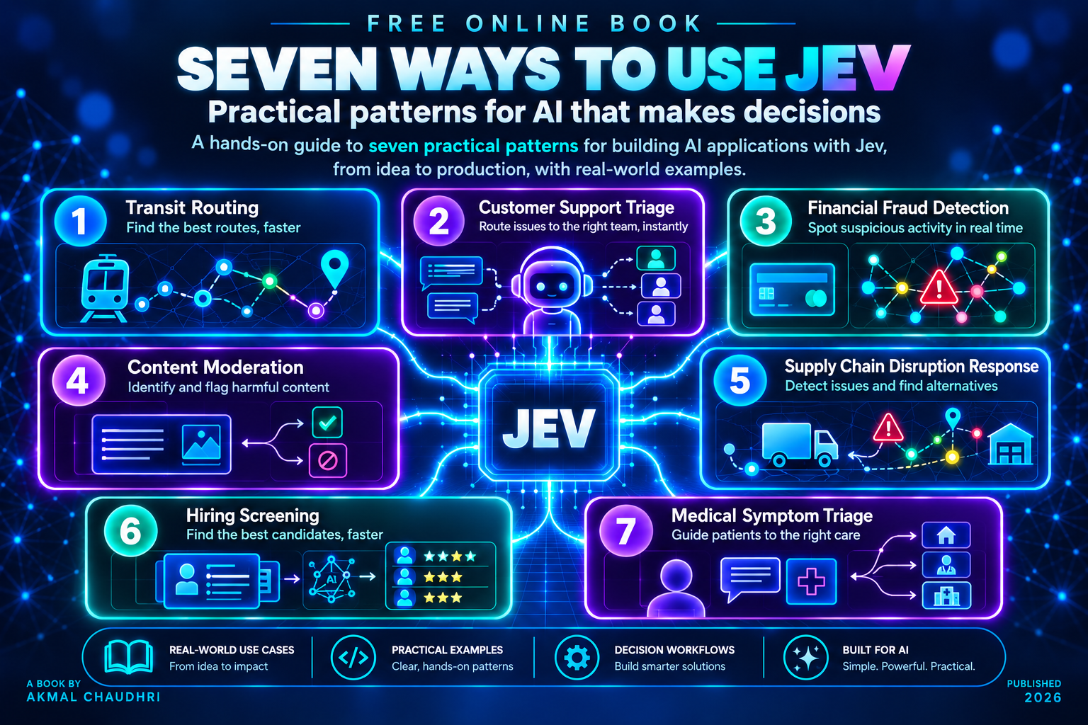
A practical guide to TypeSafe AI’s structured decision model, exploring seven domains where a single Choice call – structured state in, typed decision out, calibrated confidence alongside – replaces brittle rules-based logic. Each chapter pairs one domain with a hands-on Jupyter notebook and examines what the confidence score reveals about the decision:

Transit Routing - Northern Line branch triage using a NetworkX graph
Customer Support Triage - Ticket routing by team and priority
Financial Fraud Detection - Flag or pass with a three-tier confidence response
Content Moderation - Approve, flag or remove user-generated content
Supply Chain Disruption - Alternative supplier selection under live constraints
Hiring Screening - CV screening against a structured job description
Medical Symptom Triage - Care pathway assignment with a conservative bias

A recurring theme across all seven chapters: the confidence score is more informative than the decision itself for uncertain cases and the threshold between automatic routing and human review is always a business decision, not a technical one.

Lessons Learned Putting Jev Inside Neo4j

Read Online ↗

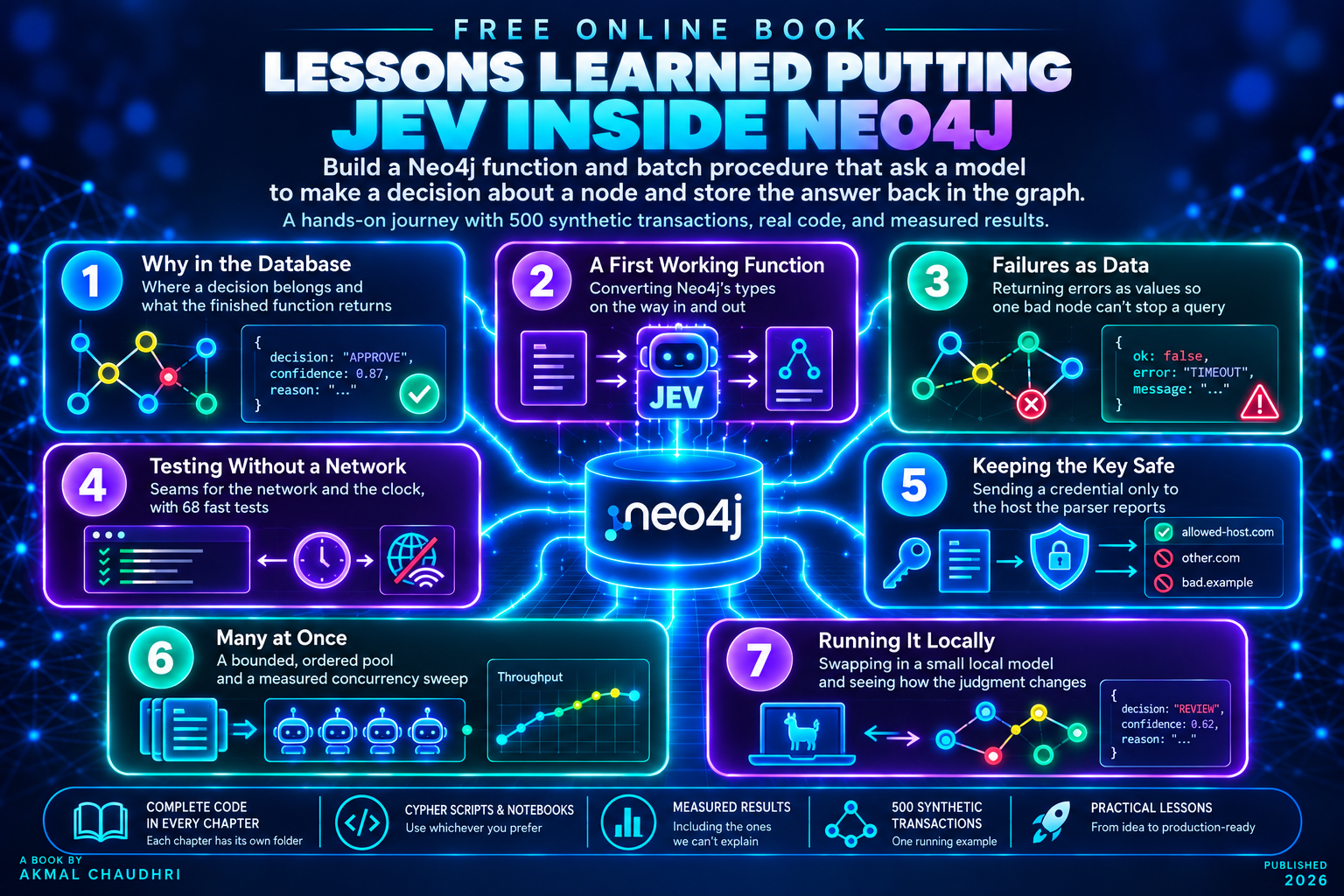
A hands-on account of building a Neo4j function and batch procedure in Java that ask a model to make a decision about a node and store the answer back in the graph. The book follows one running example, 500 synthetic transactions and each chapter adds the code that the previous chapter’s problem called for. The lessons:

Why in the Database - Where a decision belongs and what the finished function returns
A First Working Function - Converting Neo4j’s types on the way in and out
Failures as Data - Returning errors as values so one bad node can’t stop a query
Testing Without a Network - Seams for the network and the clock, with 68 fast tests
Keeping the Key Safe - Sending a credential only to the host the parser reports
Many at Once - A bounded, ordered pool and a measured concurrency sweep
Running It Locally - Swapping in a small local model and seeing how the judgment changes

Every chapter with code has its own folder in the repository and each Cypher script also comes as a notebook, so you can use whichever you prefer. The results are reported as measured, including the ones we can’t explain!

Keyboard shortcuts

Real-Time Supply Chain Routing with Neo4j, Snowflake Postgres and Confluent Kafka